Turbulence

A sequence of Jupyter notebooks featuring the "12 Steps to Navier-Stokes"

12 steps to Navier–Stokes

The interactive module 12 steps to Navier–Stokes is one of several components of the Computational Fluid Dynamics class taught by Prof. Lorena A. Barba in Boston University between 2009 and 2013.

You can see that two distinct pressure zones are forming and that the spiral pattern expected from lid-driven cavity flow is beginning to form. Experiment with different values of nt to see how long the system takes to stabilize.

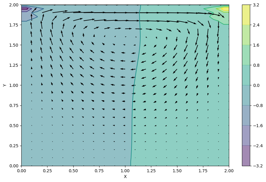
The quiver plot shows the magnitude of the velocity at the discrete points in the mesh grid we created. (We're actually only showing half of the points because otherwise it's a bit of a mess. The X[::2, ::2] syntax above is a convenient way to ask for every other point.) Another way to visualize the flow in the cavity is to use a streamplot

To use these lessons, you need Python 3, and the standard stack of scientific Python: NumPy, Matplotlib, SciPy, Sympy. And of course, you need Jupyter—an interactive computational environment that runs on a web browser.